Finding the global minimum of a complex, non-convex energy landscape is a fundamental problem in both statistical mechanics and combinatorial optimization. When we deal with “Spin Glasses” (systems with random, competing interactions), the number of possible states grows exponentially as $2^n$. For $n=100$, the state space is $2^{100}$, far beyond the reach of exhaustive search. This post explores how we can leverage the physics of thermodynamics and the Metropolis-Hastings criterion to navigate this landscape effectively.
1. The Physics: Spins and Couplings
Imagine a lattice where each site $i$ contains a magnetic “spin” $s_i$. In the Ising model, these spins are binary: they can only point UP ($+1$) or DOWN ($-1$). These spins are not isolated; they interact with their neighbors through a coupling strength $J_{ij}$.
There are two primary interaction rules:
- Ferromagnetic ($J_{ij} > 0$): The atoms want to align. If $s_i$ is $+1$, it pulls $s_j$ towards $+1$.
- Antiferromagnetic ($J_{ij} < 0$): The atoms want to be anti-aligned. If $s_i$ is $+1$, it pushes $s_j$ towards $-1$.
A system where these interactions are random and frustrated (meaning no single configuration can satisfy all couplings simultaneously) is what I call a Spin Glass.
2. The Math: The Hamiltonian
To quantify the “tension” in the system, I use the Hamiltonian ($H$), which represents the total energy. The goal of the system is to reach the state of lowest possible energy.
The Hamiltonian is defined as:
$$H = -\sum_{i < j} J_{ij} s_i s_j$$
Here, the negative sign is crucial. If $J_{ij} > 0$ (ferromagnetic) and $s_i, s_j$ are aligned ($s_i s_j = +1$), the term $-J_{ij} s_i s_j$ becomes negative, lowering the total energy. If they are anti-aligned, the energy increases.
In a computational context, I often represent $J$ as a symmetric matrix with zero diagonal ($J_{ii} = 0$). To handle the summation efficiently via linear algebra, I can rewrite the Hamiltonian as:
$$H = -\frac{1}{2} \sum_{i} \sum_{j} J_{ij} s_i s_j = -\frac{1}{2} s^T J s$$
3. The Hardware Shortcut: Local Energy Change ($\Delta E$)
Recalculating the entire Hamiltonian every time I flip a single spin is computationally expensive, $O(N^2)$. To optimize, I derive the local energy change ($\Delta E$) when flipping a single spin $s_k \rightarrow -s_k$.
Isolating the energy contribution of spin $k$:
$$E_k = -s_k \sum_{j \neq k} J_{kj} s_j$$
When I flip $s_k$, the new energy contribution is $E_{k, new} = -(-s_k) \sum J_{kj} s_j$. The difference is:
$$\Delta E = E_{k, new} - E_{k, old} = 2 s_k \sum_{j} J_{kj} s_j$$
This reduces the complexity to $O(N)$, a massive gain for both software simulations and hardware implementations.
4. The Logic: Energy Landscape and the Greedy Trap
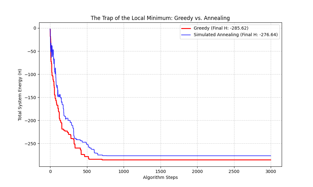
If I use a Greedy Algorithm, I only accept a spin flip if $\Delta E < 0$. While this ensures the energy always decreases, it inevitably leads to a Local Minimum.
Imagine a mountain range with many small craters. A greedy agent walking downhill will get stuck in the first crater it finds, even if a much deeper valley (the Global Minimum) exists just beyond a small ridge. Because the agent refuses to walk “uphill,” it can never escape the local trap.
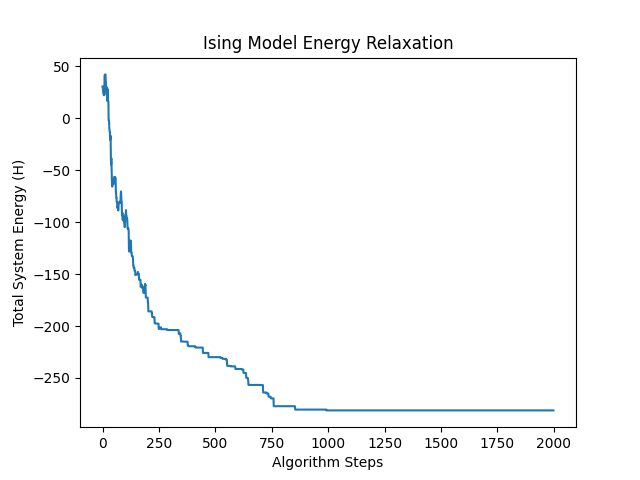
The plot above shows the energy relaxation. Notice the jagged behavior at the start: this is the system intentionally taking “bad” moves to explore the landscape before settling.
5. Thermodynamics: Simulated Annealing
To escape local minima, I introduce the concept of Temperature ($T$). In physics, temperature represents thermal noise: atomic jitter that allows spins to flip even if it increases energy.
I use the Metropolis-Hastings Criterion to decide whether to accept a flip:
- If $\Delta E < 0$, Accept the flip (100% probability).
- If $\Delta E > 0$, Accept with probability $P = e^{-\Delta E / T}$.
At high $T$, $P \approx 1$, allowing the system to bounce out of local minima (Exploration). As I slowly cool the system down ($T \rightarrow 0$), $P \rightarrow 0$, and the system settles into the deepest valley it found (Exploitation).
6. Empirical Proof: Greedy vs. Simulated Annealing
Does this actually work? To prove it, I ran a Monte Carlo simulation across 50 different “universes” (random $J$ matrices). For each universe, I compared the Greedy approach against Simulated Annealing.
In a single run, Greedy might occasionally get lucky by being dropped near a deep valley. However, over multiple trials, the statistical superiority of Simulated Annealing becomes clear.
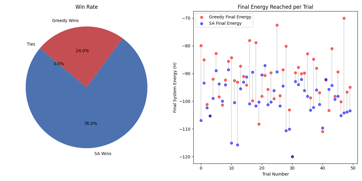
Final Tally from 50 Trials:
- Simulated Annealing Wins: 38
- Greedy Wins: 12
- Average SA Energy: -99.19
- Average Greedy Energy: -92.25
Simulated Annealing consistently finds lower energy states by refusing to be trapped by the immediate “greedy” choice. This statistical reliability is exactly why hardware accelerators for Ising models use thermal noise (or pseudo-randomness) to find global solutions to NP-hard problems.